Easy Bayesian linear modeling

STA360 at Duke University

rstanarm and bayesplot

Download

To download rstanarm and bayesplot run the code below

install.packages("rstanarm", "bayesplot")

To load the package, run

library(rstanarm)
library(bayesplot)

Overview

  • rstanarm contains a host of functions to make Bayesian linear modeling in R easy. See https://mc-stan.org/rstanarm/articles/ for a variety of tutorials.

    • pros: fast and easy to test Bayesian linear models

    • cons: limited in scope, e.g. requires differentiable objective and small model adjustments can be cumbersome to implement, e.g. placing a prior on variance versus standard deviation of normal model.

  • bayesplot contains many useful plotting wrappers that work out of the box with objects created by rstanarm in an intuitive way.

Example

library(tidyverse)
bass = read_csv(
     "https://sta101-fa22.netlify.app/static/appex/data/bass.csv")
glimpse(bass)
Rows: 171
Columns: 5
$ river   <dbl> 0, 0, 0, 0, 0, 0, 0, 0, 0, 0, 0, 0, 0, 0, 0, 0, 0, 0, 0, 0, 0,…
$ station <dbl> 0, 0, 0, 0, 0, 0, 0, 0, 0, 0, 1, 1, 1, 1, 1, 1, 1, 1, 1, 1, 1,…
$ length  <dbl> 47.0, 48.7, 55.7, 45.2, 44.7, 43.8, 38.5, 45.8, 44.0, 40.4, 47…
$ weight  <dbl> 1616, 1862, 2855, 1199, 1320, 1225, 870, 1455, 1220, 1033, 337…
$ mercury <dbl> 1.60, 1.50, 1.70, 0.73, 0.56, 0.51, 0.48, 0.95, 1.40, 0.50, 0.…

Description

Mercury, is a naturally occurring element that can have toxic effects on the nervous, digestive and immune systems of humans. In local rivers microbes transform mercury into the highly toxic methyl mercury. Fish accumulate methyl mercury (since they are unable to excrete it) in their tissue over the course of their life.

Bass from the Waccamaw and Lumber Rivers were caught randomly, weighed, and measured. In addition, a filet from each fish caught was sent to the lab so that the tissue concentration of mercury could be determined for each fish. Each fish caught corresponds to a single row of the data frame. A code book is provided below.

  • river: 0=Lumber, 1=Waccamaw
  • station that the fish was collected at
  • length of the fish in centimeters
  • weight of the fish in grams
  • mercury: concentration of mercury in parts per million (ppm)

The data come from Craig Stowe, Nicholas School of the Environment circa 1990s

Fitting a normal linear model

Let’s consider the model below:

\[ y_i = \beta_0 + \beta_1 x_1 + \beta_2 x_2 + \ldots + \beta_p x_p + \epsilon_i \]

where \(\epsilon_i \sim \text{ i.i.d.} N(0, \sigma^2)\). We complete model specification with the priors:

\[ \begin{aligned} \beta_0 &\sim N(0, 100)\\ \beta_i &\sim \text{ i.i.d } N(0, 1) \text{ for all } i > 0\\ \sigma &\sim \text{uniform}(0, \infty) \end{aligned} \]

Let’s look at building this model using the stan_glm function of rstanarm.

Note

We’ll always want to access the object we create, so you should save the result, e.g. model1 below.

# save the result as "model1"
model1 = stan_glm(mercury ~ ., data = bass, # remove the intercept
                 family = gaussian(link = "identity"),
                 seed = 360, # sets a random starting seed
                 prior_intercept = normal(0, 100), # sets the intercept prior
                 prior = normal(0, 1), # sets the beta prior
                 prior_aux = NULL, # set a flat prior on sigma
                 ) 

Examining the output

  • Did stan_glm do what we think it did? Did the Markov chain converge?
summary(model1)

Model Info:
 function:     stan_glm
 family:       gaussian [identity]
 formula:      mercury ~ .
 algorithm:    sampling
 sample:       4000 (posterior sample size)
 priors:       see help('prior_summary')
 observations: 171
 predictors:   5

Estimates:
              mean   sd   10%   50%   90%
(Intercept) -1.4    0.3 -1.9  -1.4  -1.0 
river       -0.5    0.2 -0.8  -0.5  -0.3 
station      0.1    0.0  0.1   0.1   0.1 
length       0.1    0.0  0.0   0.1   0.1 
weight       0.0    0.0  0.0   0.0   0.0 
sigma        0.6    0.0  0.5   0.6   0.6 

Fit Diagnostics:
           mean   sd   10%   50%   90%
mean_PPD 1.2    0.1  1.1   1.2   1.3  

The mean_ppd is the sample average posterior predictive distribution of the outcome variable (for details see help('summary.stanreg')).

MCMC diagnostics
              mcse Rhat n_eff
(Intercept)   0.0  1.0  2864 
river         0.0  1.0  1857 
station       0.0  1.0  1828 
length        0.0  1.0  2814 
weight        0.0  1.0  2861 
sigma         0.0  1.0  2819 
mean_PPD      0.0  1.0  3069 
log-posterior 0.0  1.0  1616 

For each parameter, mcse is Monte Carlo standard error, n_eff is a crude measure of effective sample size, and Rhat is the potential scale reduction factor on split chains (at convergence Rhat=1).
prior_summary(model1)
Priors for model 'model1' 
------
Intercept (after predictors centered)
 ~ normal(location = 0, scale = 100)

Coefficients
 ~ normal(location = [0,0,0,...], scale = [1,1,1,...])

Auxiliary (sigma)
 ~ flat
------
See help('prior_summary.stanreg') for more details
mcmc_trace(model1)

mcmc_hist(model1)

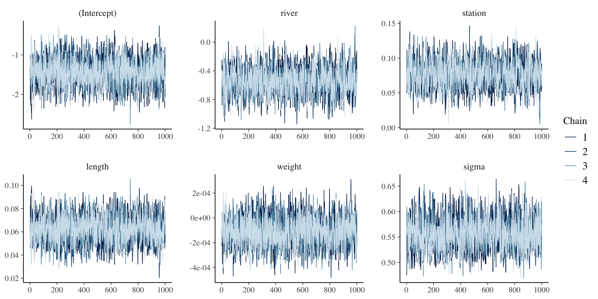
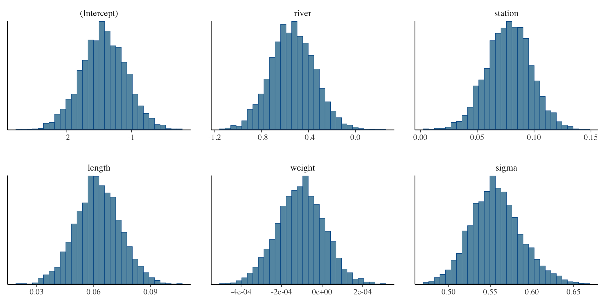
To plot specific parameters, use the arguemnt pars, e.g.

  • mcmc_trace(model1, pars = c("river", "station")
  • mcmc_hist(model1, pars = "length")

To read more about bayesplot functionality, see https://mc-stan.org/bayesplot/articles/plotting-mcmc-draws.html

df = data.frame(yhat = model1$fitted.values,
                residual = model1$residuals)

df %>%
  ggplot(aes(x = yhat, y = residual)) +
  geom_point() +
  theme_bw()

chain_draws = as_draws(model1)
print(names(chain_draws))
[1] "(Intercept)" "river"       "station"     "length"      "weight"     
[6] "sigma"       ".chain"      ".iteration"  ".draw"      
chain_draws$river[1:5] # first 5 samples of the first chain run by stan
[1] -0.3748586 -0.2472218 -0.8788921 -0.4870408 -0.6565987
  • try the following command: View(chain_draws)

Report posterior mean, posterior median and 90% posterior CI.

posteriorMean = apply(chain_draws[,1:6], 2, mean)
posteriorMedian = model1$coefficients
posteriorCI = posterior_interval(model1, prob = 0.9)
cbind(posteriorMean, posteriorMedian, posteriorCI)
            posteriorMean posteriorMedian            5%           95%
(Intercept) -1.4320242215    -1.435098280 -2.0129526891 -8.767706e-01
river       -0.5368486696    -0.538925449 -0.8441961657 -2.299097e-01
station      0.0777090920     0.078115486  0.0461303215  1.092244e-01
length       0.0622405968     0.062062419  0.0429862421  8.203404e-02
weight      -0.0001059707    -0.000104737 -0.0002995203  8.105592e-05
sigma        0.5568710635    -1.435098280  0.5088456218  6.111942e-01

Exercise: Bayesian logistic regression

Using the bass data set, see how well you can predict which river a bass came from, given only its length and mercury level. In other words,

\[ p(y_i = 1) = \frac{1}{1 + \exp [- (\beta_0 + \beta_1 x_1 + \beta_2 x_2)]} \]

Use the priors

\[ \beta_i \sim N(0, 4) \text{ for } i \in (0, 1, 2) \]

A template for fitting logistic regression using rstanarm can be found at https://mc-stan.org/rstanarm/articles/binomial.html.

  • Does your chain converge?
  • Report \(E[\beta_i | y]\) and 80% posterior CI for each \(\beta\), i.e. \(i \in (0, 1, 2)\)
  • Is length or mercury a more important predictor of which river the bass came from? Why?